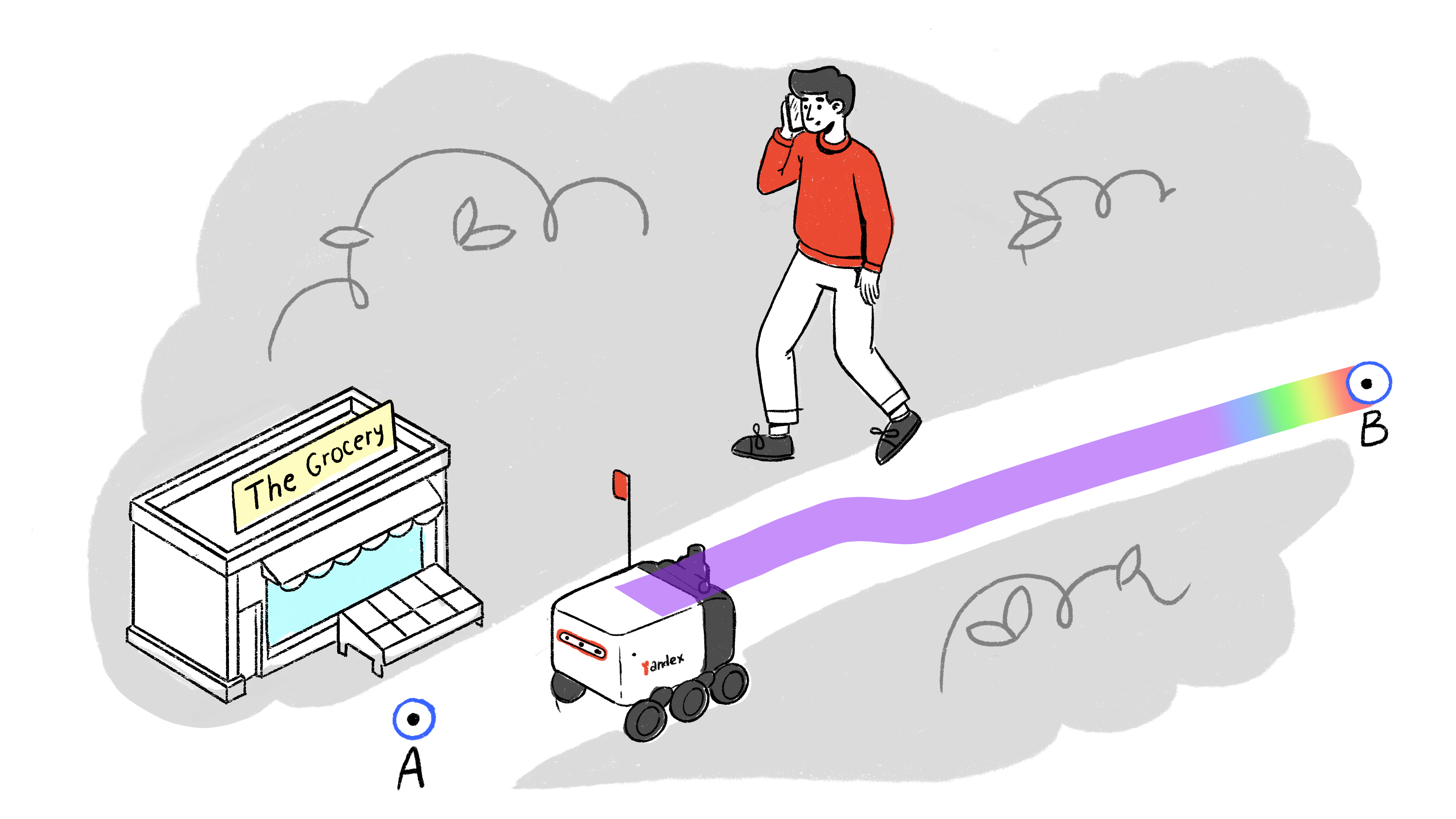
Almost 2 years ago, in Dec’22, I started working as a Computer Vision Engineer in the perception team for a food delivery robot. After working on talking face geneations in the past, my main desire was to work on something that would impact the real world. The food delivery robot running on the streets of Moscow seemed like a perfect match, and it definitely was. However, while my dream came true, I also found myself immersed in a product so complicated I’d never expected.
There are a lot of things to discuss: hardware, simulator, remote operators, and more. But today, I want to focus on the part closest to me – the technology onboard that runs in real-time whenever the robot is in motion. But first, let’s discover what this delivery robot actually is.
The idea behind this robot is to automate last-mile delivery. Whenever you order food from a restaurant or groceries from a store, imagine a robot that will autonomously deliver it to you.
That’s how it works nowadays on the streets of Moscow, St. Petersburg, Sochi, and Innopolis in Russia, as well as in Almaty, Kazakhstan. Of course, we still have human couriers, but robots are becoming more popular every day.

Our fleet operates continuously, even during the harsh Russian winters, which can be quite challenging. Thankfully, people love and support our robots 🥹
As you see on the video above, one of the main challenges is constantly changing conditions, from unpredictable weather to sudden construction sites blocking paths. The biggest challenge, though, is people. While drivers in vehicles tend to be more predictable as they follow traffic rules, pedestrians can behave in truly unexpected ways..
But let’s return to the subject, and explore how our robot tackles these challenges through its core technology stack.
The delivery robot’s architecture consists of five key components:
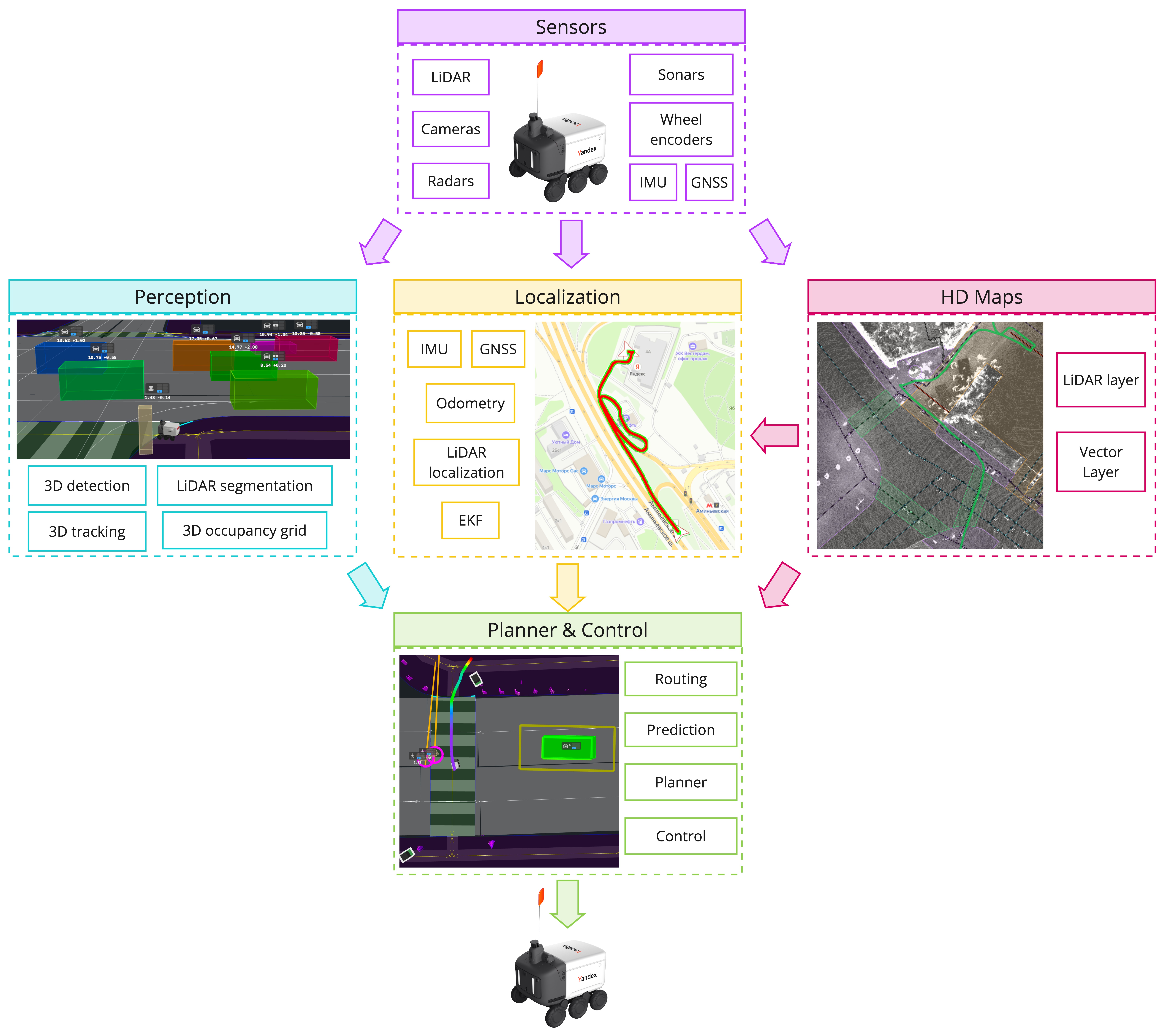
The sensors installed on the delivery robot can be divided into two groups: those for perceiving the surrounding world and those for determining the robot’s position within it. The first group includes sensors that help scan the environment and recognize objects, such as lidars, cameras, radars, and sonars. The second group includes sensors that track the robot’s position, speed, and orientation: IMU, GNSS, and wheel encoders.
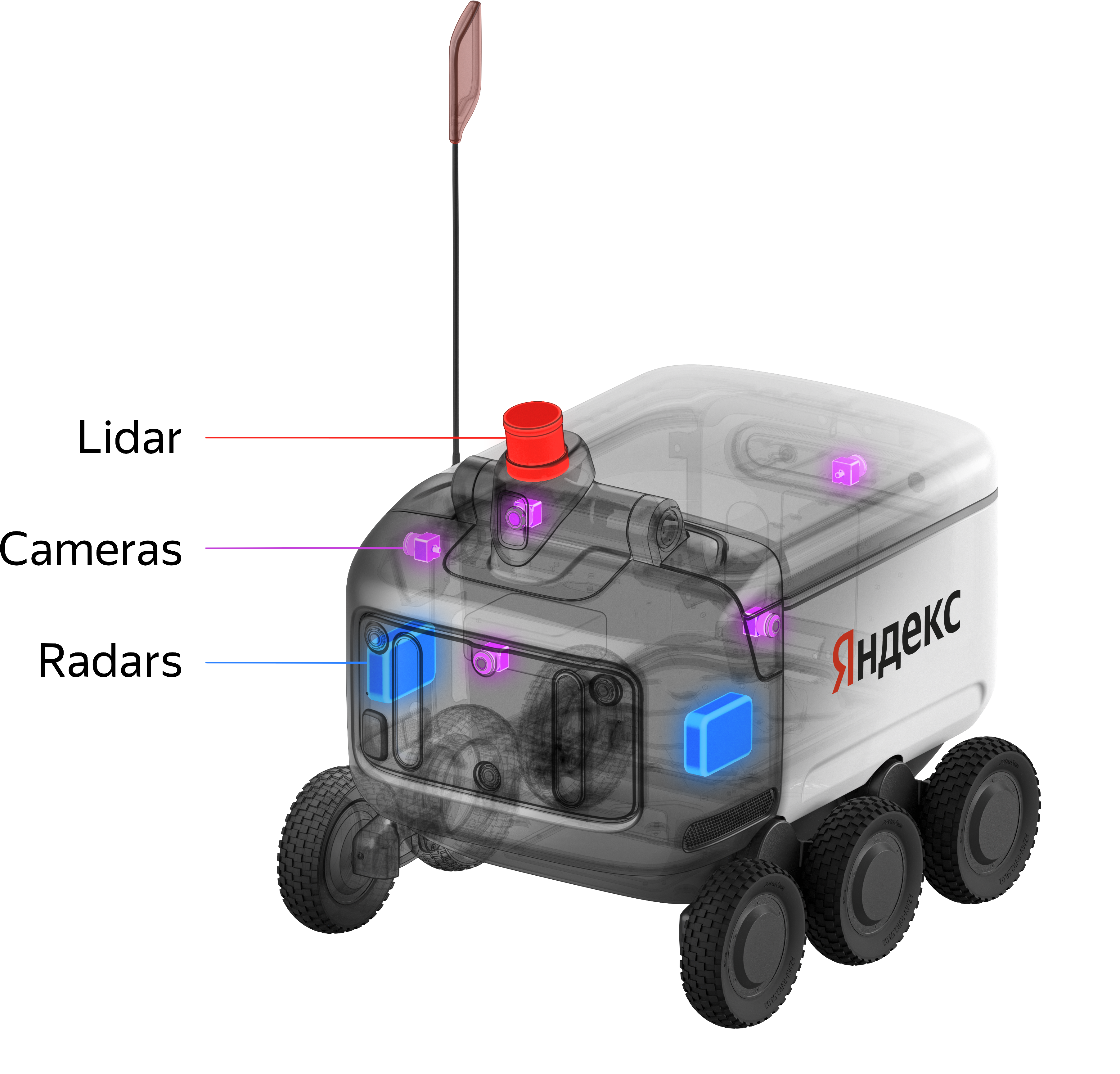
LiDAR (Light Detection and Ranging) measures distances by emitting laser pulses and timing their return after reflecting off objects.

Our 64-beam LiDAR generates a detailed 3D point cloud, scanning up to 30 meters. Thanks to the high density of data, we can not only accurately measure the distance to objects but also easily classify them based on their shape.
To learn more about LiDAR technology, check out this overview from Hesai, a leading global manufacturer of LiDAR sensors.
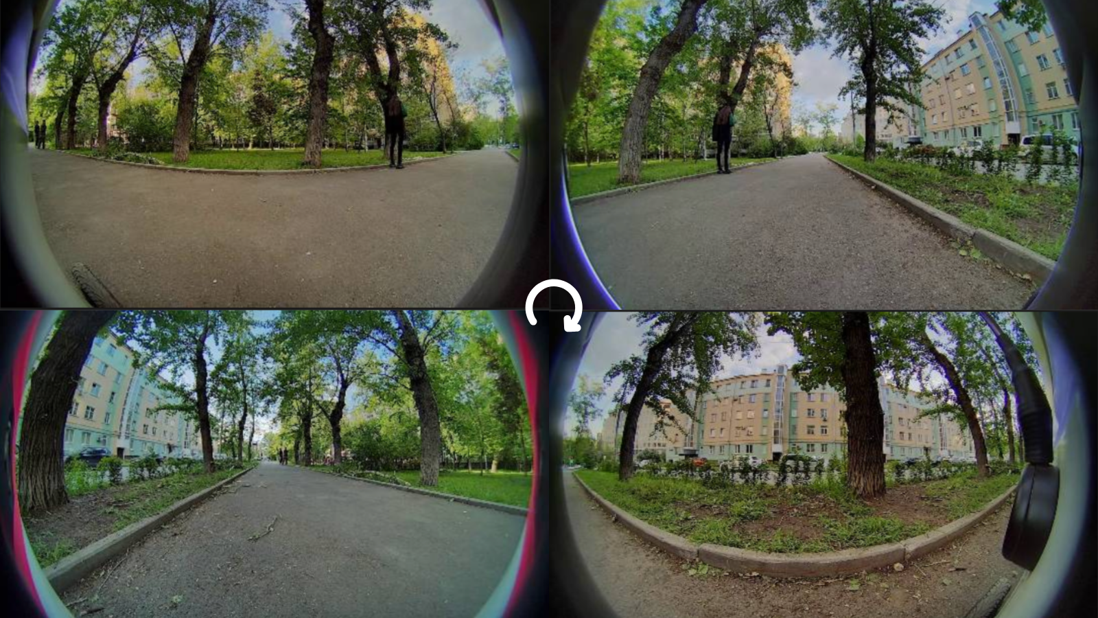
The robot is also equipped with four fisheye cameras, strategically positioned to provide a complete 360-degree view without blind spots. Our image processing pipeline transforms these fisheye images into a spherical projection. This transformation enables us to seamlessly combine all camera frames into an undistorted panoramic view. For those interested in the technical details of fisheye image projection, you can learn more here.
Radar complements the LiDAR by using radio waves to detect and measure the speed of objects up to 150 meters away. It relies on the Doppler effect, which allows it to accurately determine an object’s velocity. This capability is especially valuable when the robot approaches crosswalks, as the radar can detect oncoming vehicles from a greater distance and precisely estimate their speed.
Sonars use ultrasonic waves to detect nearby objects, typically within 1-2 meters. These sensors emit high-frequency sound pulses and measure the time it takes for the echoes to return, providing precise distance measurements for very close obstacles. This adds an extra layer of safety, especially in tight spaces or when maneuvering around pedestrians.
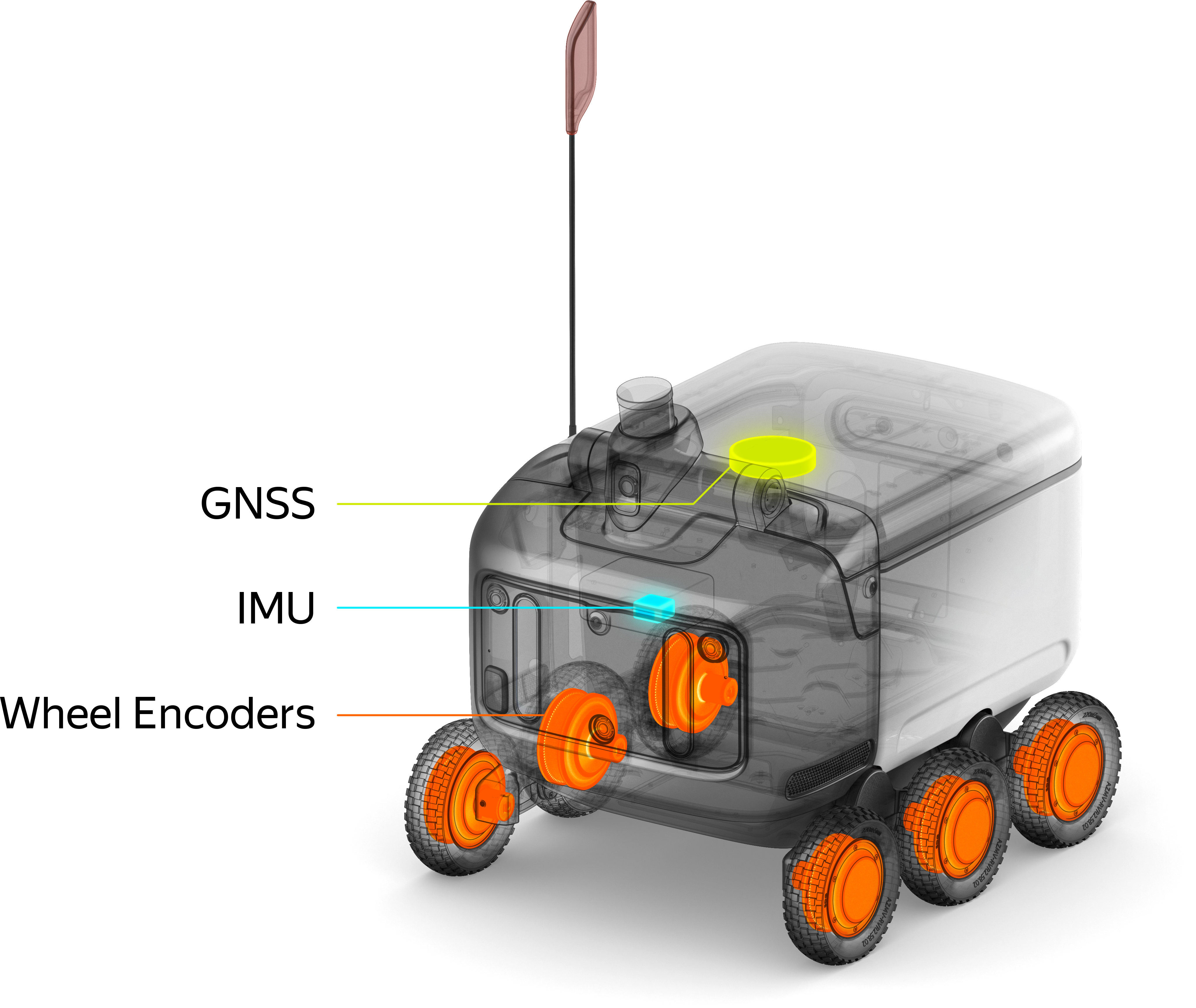
GNSS (Global Navigation Satellite System) determines the robot’s location on Earth. This global satellite navigation system combines multiple satellite networks, including GPS (USA), GLONASS (Russia), Galileo (Europe), and BeiDou (China).
IMU (Inertial Measurement Unit) is a compact device housing both an accelerometer and a gyroscope. It allows determining the robot’s linear acceleration and angular velocity.
Wheel Encoders are high-precision sensors installed on the robot’s wheels. They register the slightest wheel rotations, allowing accurate measurement of distance traveled and movement speed.
With an understanding of the data these sensors provide, let’s explore how our algorithms process this information.
The perception system’s primary goal is to identify objects around the robot that could impact its movement. These objects fall into two categories: dynamic (such as people, cars, and scooters) and static (like buildings, poles, and trees).
For dynamic objects, the system focuses on accurately predicting their direction and speed. Such accurate forecasting enables the robot to respond swiftly and appropriately, whether it’s adjusting its path for an oncoming car or yielding to a fast-moving scooter.
When it comes to static objects, the emphasis is on determining their size. Precise recognition of static objects is essential for the robot to navigate safely, especially in tight spaces like narrow sidewalks where it needs to maintain a safe distance from building walls.
The delivery robot employs two key techniques to perceive its surroundings: 3D object detection and 3D occupancy grid mapping. The 3D detection capability allows the robot to identify the type of each dynamic object, pinpoint its exact location, measure its dimensions, and calculate its direction and speed. Meanwhile, the occupancy grid divides the space into small 5x5 cm cells, each containing information about the type of occupancy and the height of any obstacles present.
Here’s an example to illustrate how this works:
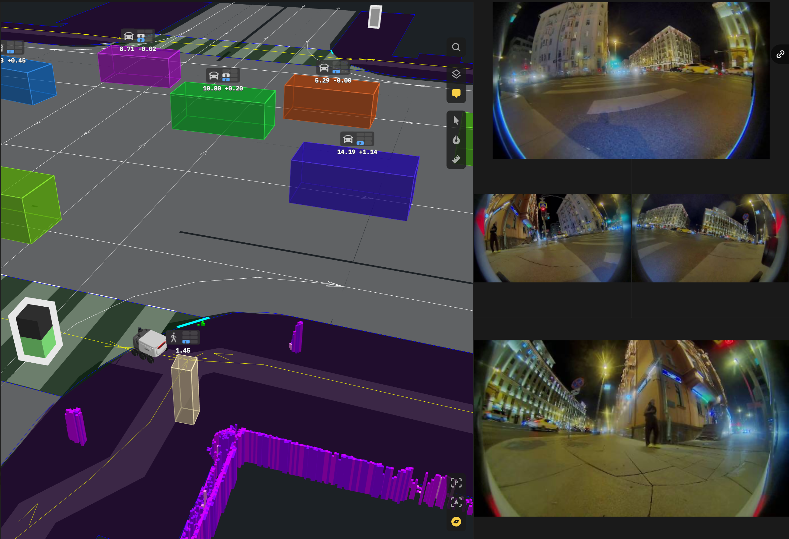
The image above illustrates the robot’s perception at a pedestrian crosswalk. On the left, we see a 3D visualization of the robot’s understanding of its surroundings. On the right are the raw camera feeds from four directions (front, left, right, and rear)
In the 3D visualization, purple columns represent the occupancy grid for static obstacles. These columns outline the shape of the building behind the robot and mark the positions of nearby objects like traffic lights and road signs.
Dynamic objects are highlighted with colorful 3D boxes, each annotated with its class, speed, and acceleration. This visualization reveals cars moving on the adjacent road and a pedestrian approaching from behind the robot. and acceleration. This reveals cars on the adjacent road and a pedestrian approaching from behind the robot.
Let’s break down how we create those colorful boxes and purple columns. We process data from cameras and lidar in four main steps:
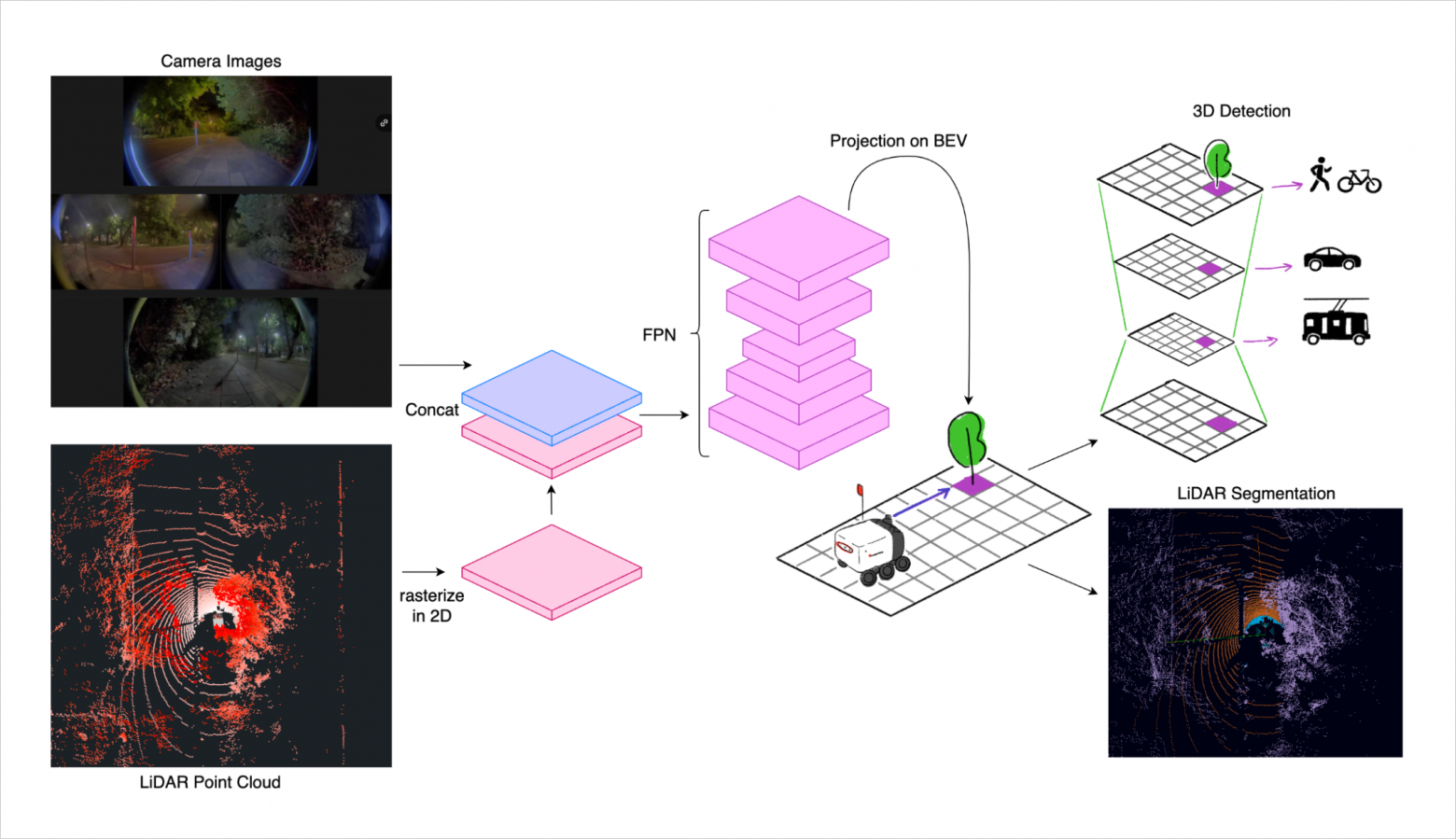
As a result, we obtain 3D object detections and LiDAR point segmentation. A tracking system then matches these newly detected objects with previously known ones using the Hungarian algorithm.
This tracker continuously updates each tracked object’s information, including its position, speed, and movement direction. It creates new tracks for newly detected objects, ensuring all objects around the robot are monitored, even if they briefly disappear from view.
We also combine predicted occupancy grids over time using a Bayes filter. This filter updates the probability of each grid cell being occupied based on new predictions. As a result, we get a more accurate picture of static obstacles around the robot.
Perception helps the robot move safely by interpreting its surroundings. But for good navigation, it also needs a bigger picture. That’s where HD maps help.
High Definition (HD) maps serve as the robot’s detailed digital blueprint of the world. These maps consist of two key components:
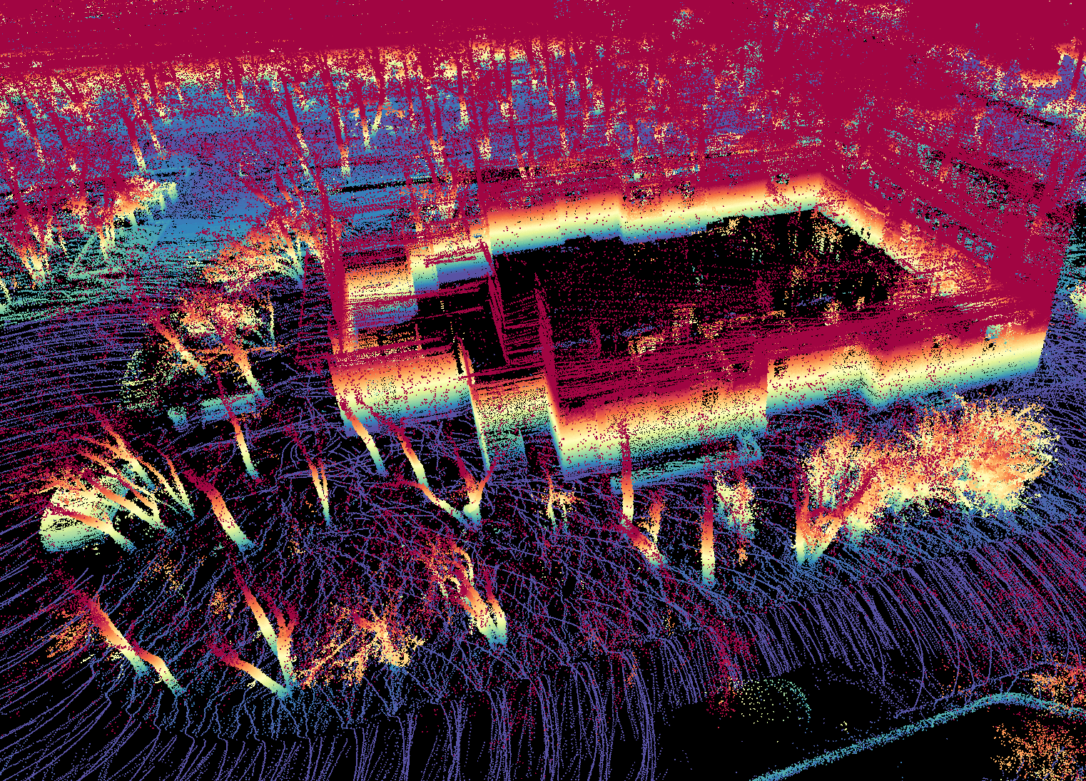
The LiDAR layer of our HD maps forms a detailed three-dimensional model of the environment, consisting of a dense point cloud anchored to absolute coordinates.
Creating this layer is a straightforward, automated process. We simply drive once along all sidewalks and pedestrian paths in the target area, collecting data in manual mode. This data is then processed through an optimization algorithm, resulting in a dense point cloud suitable for localization. For efficiency, we can even use autonomous taxis to capture data for sidewalks adjacent to roads, as their LiDAR systems are equally capable of generating the required point clouds.
To ensure the stability and consistency of our maps, we apply filtering techniques to remove points associated with dynamic objects such as cars or pedestrians. This filtration process relies on our advanced perception system for accurate object detection. The result is a robust foundation for robot localization that remains reliable over time, even as the urban environment experiences minor changes.
The vector layer of our HD maps is meticulously crafted by cartographers using LiDAR data and camera imagery. This layer encodes crucial information about the robot’s operational environment, delineating movement zones such as pedestrian crossings, sidewalks, bike paths, and mixed-use areas like parking lots or courtyards.
Beyond simple boundaries, the vector layer captures the intricate network of traffic lights, including their positions, interconnections, and the specific maneuvers they control. This comprehensive traffic light data enables our robots to anticipate signal changes even when direct visual confirmation is obstructed by people or vehicles.
To further enhance navigation, the vector layer incorporates dedicated lanes for robot movement, bicycle paths for predicting cyclist behavior, and projected vehicle trajectories. This rich dataset empowers our robots to plan safe, efficient routes while accounting for the complexities of urban landscapes and the anticipated behaviors of other road users.
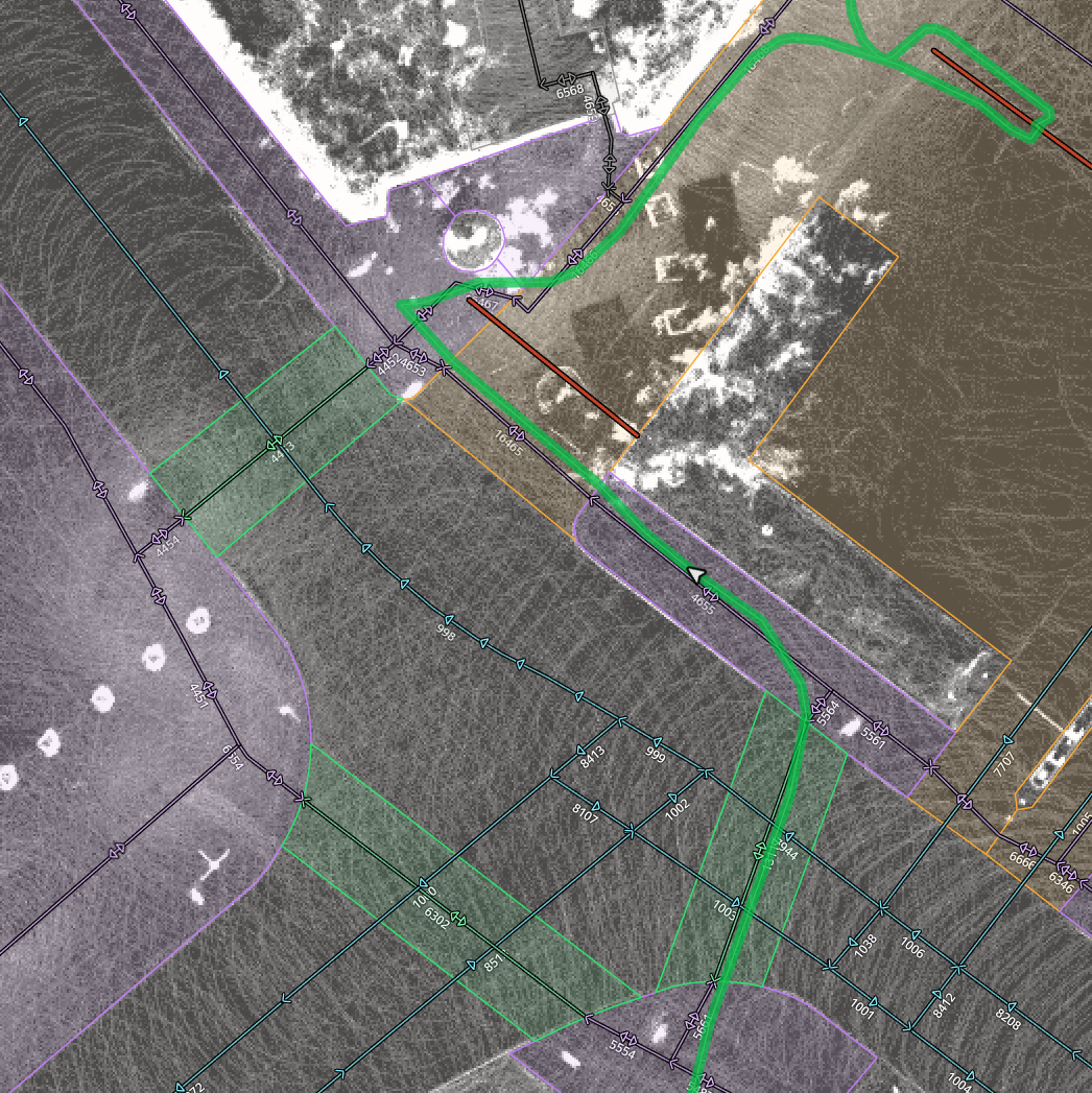
Precision is paramount in our mapping process. Our vector layer achieves centimeter-level accuracy for every object, exceeding commercial HD map capabilities. Therefore, we are working to simplify vector map creation through data streamlining, format simplification, and ML-driven automation, shifting some detection tasks to onboard perception.
The vector layer reduces onboard computing needs and simplifies perception tasks. However, it requires precise localization to be effective. Our localization module provides this capability, allowing robots to accurately position themselves within the detailed map.
The main goal of localization is to determine the robot’s position, orientation, speed, and acceleration in its environment. To achieve this, we combine data from various sensors:
We also employ LiDAR localization, which determines the robot’s position by comparing the current LiDAR snapshot to the LiDAR layer from our HD map. Using the example of Yandex’s favorite horse, the source data might look like this:
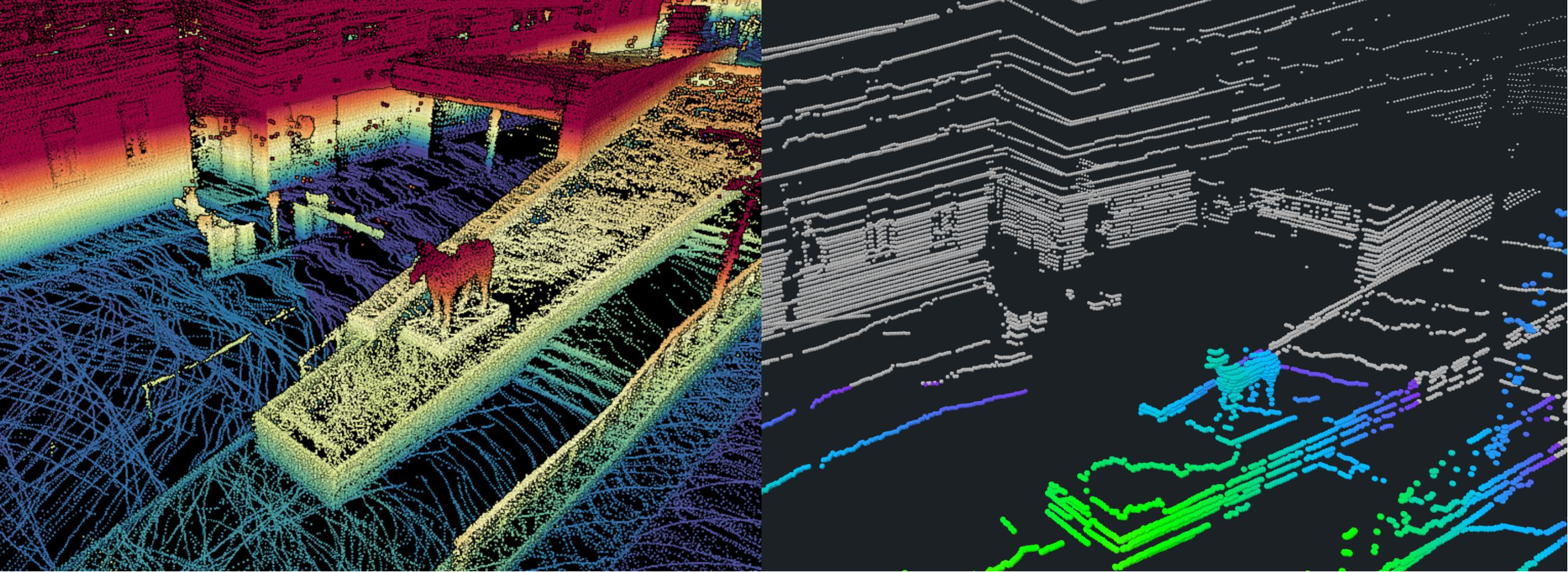
This task is called point-cloud registration, and there are many algorithms to solve it. In our case, the robot uses the NDT (Normal Distribution Transform) algorithm. Here’s how it works:
The LiDAR layer of the HD map is preprocessed by dividing all three-dimensional space into cells. For cells containing LiDAR points, a surface model is constructed to describe these points. This model approximates the surface with an ellipsoid, and each cell stores the model parameters and the coordinates of the central point.
Before applying the NDT algorithm, the robot’s LiDAR point cloud is also preprocessed. Points belonging to the robot itself and dynamic objects are removed. To optimize computations, a reference subset of points is selected from the entire cloud.
It’s important to note that the algorithm requires an initial approximation of the robot’s position to work correctly, as it’s only effective within a limited radius around the actual position.
For each new LiDAR point cloud, the algorithm performs the following actions:
While this method allows for accurate determination of the robot’s position, it can face challenges in environments lacking distinctive features, such as empty parking lots. Similarly, areas with uniform buildings can cause confusion, potentially leading the algorithm to mistake one side of a building for another.
Considering that each localization method has its own errors, we use the Extended Kalman Filter (EKF) to combine readings from all sensors and obtain the most accurate result.
What features of our task make EKF a suitable solution?
To properly account for both absolute knowledge about localization and information about relative movement, EKF performs two actions at each cycle. First, it predicts the robot’s new position, as well as parameters of speed, acceleration, and orientation based on the known previous state of the robot and a certain motion model. Second, it updates the prediction using data from sensors and LiDAR localization. The resulting estimate becomes the starting point for the next EKF cycle.
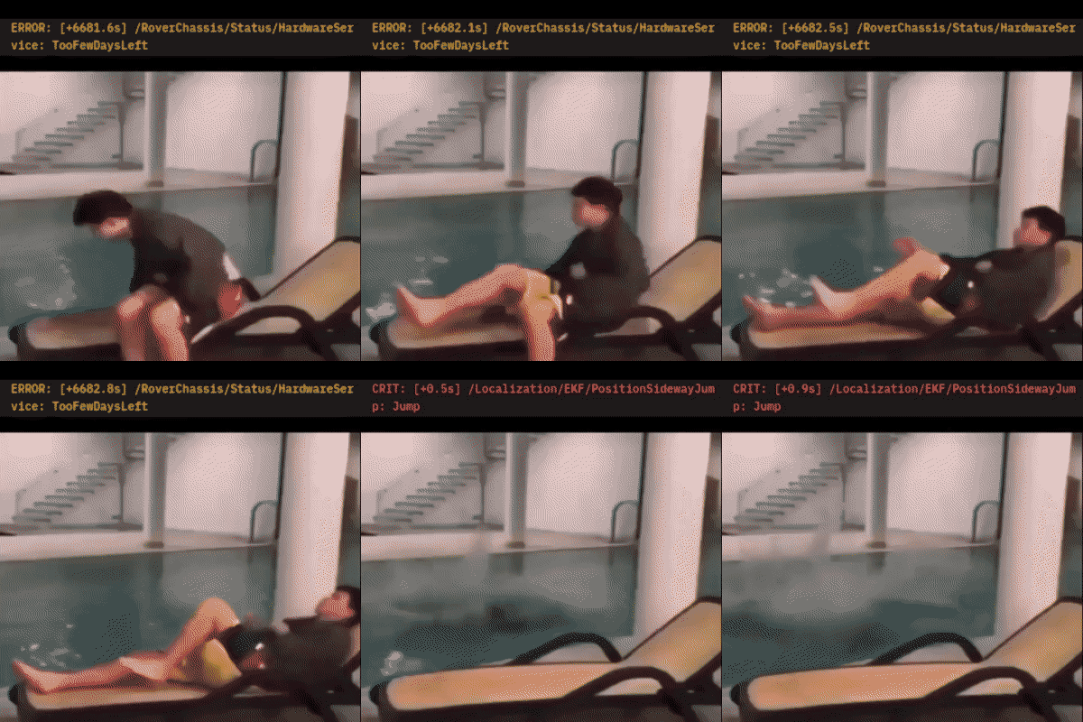
In theory, it sounds good and reliable, but in practice, EKF requires proper parameter tuning: which method to trust more in which situation. Incorrect calibration can lead to instabilities, resulting in “jumps” in localization.
Once the perception, localization, and HD map components have provided a comprehensive view of the environment, the focus shifts to planning and controlling the delivery robot’s movement. The motion planner takes this information to construct an optimal route and predict potential trajectories of other participants. Meanwhile, the control system ensures the robot follows this route precisely, making real-time adjustments to its movement as needed.
The delivery robot’s journey begins when it receives two locations from a backend service: where to pick up the order and where to deliver it. The robot then plans its route using HD map data, considering road infrastructure (crosswalks, sidewalks, bike paths) and potential obstacles (roadworks, snow drifts, narrow passages). We also account for other delivery robots’ locations and planned routes to avoid conflicts in tight spaces.
To find the best path, we transform this information into a weighted graph. The A* algorithm then calculates the optimal route through this graph, efficiently navigating the robot from pickup to delivery point.
With our global route established, we’re ready to move. We already know about static obstacles from our HD maps and have just received fresh information from the perception. We’re also aware of other road users’ positions and speeds.
However, this isn’t enough. To plan a safe path, we need to anticipate where these dynamic objects might go, ensuring our movement doesn’t interfere with theirs. That’s why we attempt to predict possible trajectories for each dynamic object. Our motion prediction system helps us with this task.
Currently, this system consists of a complex set of rules that rely on information from the tracker (object class, direction, and speed) and data from HD maps (such as the lane graph, which represents possible paths for vehicles and pedestrians).
After evaluating all potential obstacles, the robot proceeds to plan its local route — typically for the next 20 meters along the global path. This process involves two key components:
As with the global route planning, the A* algorithm is also used here, but with additional factors taken into account: the robot’s physical limitations, people and vehicles crossing its path, static objects, speed limits for safety considerations, and other parameters.
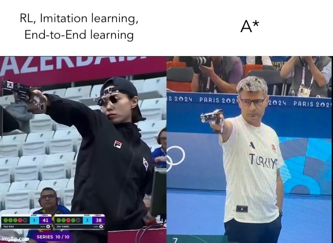
While we’re actively exploring various ML approaches, the classic A* algorithm continues to perform reliably for our needs.
After constructing the trajectory, following it precisely is challenging due to various factors: road irregularities, changing friction, and incomplete sensor data. These errors can throw the robot off course, necessitating a control system for continuous movement adjustment.
Our approach to controlling the delivery robot includes two main components:
I won’t go into the details of these control algorithms here, as they warrant their own thorough discussion. However, if you’re curious to learn more, check out this excellent wiki page. It provides in-depth coverage of PID control, the kinematic bicycle model, and the Pure Pursuit algorithm.
In summary, the Control component ensures precise decision-making at all levels, from global route planning to local maneuvering. This allows our delivery robot to navigate efficiently and safely through various environments and situations.
Whew! That turned out to be quite a long story - thanks for sticking with me until the end! While I’ve covered the main components of our delivery robot’s technology, there’s still so much more under the hood: sensor calibration systems, traffic light detection, specialized detectors (like our pit detection system), and privacy features like face and license plate blurring. One hopes that end-to-end solutions will come, and future developers won’t need so much stuff xD
Tranks to Victor Yurchenko, Alexander Ivanov, Sergei Stradomskii, Alexey Golomedov, Olesia Krindach, Leonid Grechishnikov и Alexander Smirnov for reading drafts of this article.