DETR: End-to-End Object Detection with Transformers (ECCV 2020)

Sun, 11 Jun 2023

Main ideas

drop multiple hand-designed components that encode prior knowledge, like spatial anchors or NMS, by treating object detection as a direct set prediction problem
new powerful architecture: the conjunction of the bipartite matching loss and transformer with (non-autoregressive) parallel decoding

How does it work?

Two ingredients are essential for direct set predictions in detection:

a set prediction loss that forces unique matching between predicted and ground truth boxes
an architecture that predicts (in a single pass) a set of objects and models their relation

Loss

DETR infers a fixed-size set of $N$ predictions ($N$ significantly larger number of object in an image). The GT set of objects is padded to $N$ by the background (no object $\varnothing$ class).

Each GT element looks like a $y_i = (c_i, b_i)$, where $c_i$ is the target class label (which may be $\varnothing$) and $b_i \in [0, 1]^4$ is a vector that defines ground truth box center coordinates, height and width relative to the image size.

Let’s define the bounding box loss as a linear combination of the $l_1$ loss (which is not scale invariant) and the generalized IoU loss (scale-invariant), these two losses are normalized by the number of objects inside the batch: $$L_{box}(b_i, b_{\sigma(i)}^{pred}) = \lambda_{iou} L_{iou}(b_i, b_{\sigma(i)}^{pred}) + \lambda_{L_1}\Vert{b_i - b_{\sigma(i)}^{pred}}\Vert_1 ,$$ where $L_{iou}(b_i, b_{\sigma(i)}^{pred}) = 1 - L_{giou}(b_i, b_{\sigma(i)}^{pred})$.

First of all, we want to find one-to-one matching for the predictions and GT-boxes. The naive solution of sorting each set by coords (top to bottom, left to right) is bad, because it can incorrectly assign hypothesis-candidates to ground instances when the model produces false positives or false negatives.

The proposed solution is to use Hungarian algorithm with following comparison function (aka matching cost): $$L_{match}(y_i, y_{\sigma(i)}^{pred}) = - p_{\sigma(i)}^{pred}(c_i) + L_{box}(b_i, b_{\sigma(i)}^{pred}) \text{ if } c_i \notin \varnothing \text{ else } 0,$$ where $\sigma$ is current permutation of elements, $p$ – the probability of class $c_i$.
The cost matrix is calculated for all possible pairs, and then a Hungarian algorithm is used to find the optimal assignment (with the lowest cost) of predicted boxes to ground truth boxes: $$\sigma_{optimal} = \underset{\sigma}{\text{argmin}} \sum_{1}^{N}L_{match}(y^i, y_{pred}^{\sigma(i)}).$$

The second step is to calculate the loss function (called Hungarian loss, the name of which can be confusing because it is used after the Hungarian algorithm itself) for the optimal assignment, which is defined as a linear combination of a negative log-likelihood for class prediction and a box loss: $$L_{hungarian}(y, y^{pred}) = \sum_{1}^{N}[- \log p_{\sigma_{opt}(i)}^{pred}(c_i) + \mathbb{1}\{c_i \neq \varnothing\}L_{box}(b_i, b_{\sigma_{opt}(i)}^{pred})],$$ where $\sigma_{opt}$ – the optimal assignment, the log-probability term down-weight by a factor 10 when $c_i = \varnothing$. Notice that the matching cost between an object and $\varnothing$ doesn’t depend on the prediction.

Architecture

I like huggingface overview of architecture.

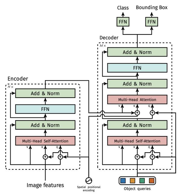
DETR’s transformer in details:

There are some interesting points I want to mention:

The transformer encoder expects a sequence as input, they give it a feature map $ d × HW$. That is, one feature is like one point, and attention is like a combination of two points that perfectly describes the bounding box.
The decoding of the output is non-autoregressive and parallel.
DETR uses so-called object queries to detect objects in an image, which are initialised with zeros and their number is is usually set to 100 means if an image only contains 4 objects, 96 annotations will just have a “no object” as class and “no bounding box” as bounding box.
During training, they add FFNs predictions and Hungarian losses after each decoder layer.

Some technical details

About training:

used scale augmentation by resizing the input images such that the shortest side is at least 480 and at most 800 pixels while the longest at most 1333
applied random crop augmentations during training
all transformer weights are initialized with Xavier init
the backbone is with ImageNet-pretrained ResNet model with frozen batchnorm layers
AdamW with the initial transformer’s learning rate to $10^{−4}$, the backbone’s to $10^{−5}$, and weight decay to $10^{−4}$
applied gradient clipping, with a maximal gradient norm of 0.1
training lasted 300 epochs with a learning rate drop by a factor of 10 after 200 epochs
$\lambda_{L_1} = 5$ and $\lambda_{iou} = 2$

About the model:

tested two different ImageNet-pretrained backbones: a ResNet50 and a ResNet-101
runs at 28 FPS, similarly to Faster R-CNN-FPN with the same backbone
to be comparable in the number of parameters they chose a model with 6 transformer and 6 decoder layers of width 256 with 8 attention heads; like Faster R-CNN with FPN this model has 41.3M parameters, out of which 23.5M are in ResNet-50, and 17.8M are in the transformer

Results

It achieves significantly better performance on large objects than Faster R-CNN, likely thanks to the processing of global information performed by the self-attention. However, it obtains lower performances on small objects.

By using global scene reasoning, the encoder is important for disentangling objects. The visualisation of the attention maps of the last encoder layer of a trained model shows that encoder seems to separate instances already, which likely simplifies object extraction and localization for the decoder.

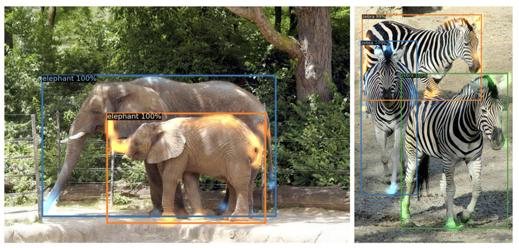
Whereas for the decoder the visualisation below shows that decoder attention is fairly local, meaning that it mostly attends to object extremities such as heads or legs. This may be because once the encoder has separated instances via global attention, the decoder only needs to attend to the extremities to extract the class and object boundaries.

Can be used for panoptic segmentation by adding a mask head on top of the decoder outputs, more precisely by adding a mask head which predicts a binary mask for each of the predicted boxes. To predict the final panoptic segmentation they used an argmax over the mask scores at each pixel, and assign the corresponding categories to the resulting masks.